Heavy Tailed Distributions and the States of Randomness

By Mellivora | 24 June 2020 | Comments 1 comment
Epistemic Status: 4/4 - Maximum Effort

Sections:
I. Normality
II. Portioning
III. Tail Terminology
IV. Mandelbrot’s Seven States of Randomness
V. Compression
VI. The Borderline
VII. Transformation Family
VIII. The Wilderness
IX. Getting More Aggressive
X. The Liquids of Randomness
XI. Stability
XII. Conclusion

I. Normality

The “Normal Distribution” (also called the Gaussian Distribution) is a very useful and well-studied tool for analysing data. It is however often misapplied, despite the efforts of Benoit Mandelbrot and Nassim Taleb to raise awareness of areas where it might be inappropriate to use. One reason people may be tempted to overuse it might be its name, which is a little too suggestive of it being some kind of “standard”, so henceforth I will use its alternative name to avoid perpetuating this any more than is inevitable.

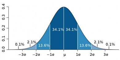
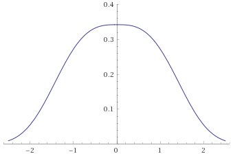
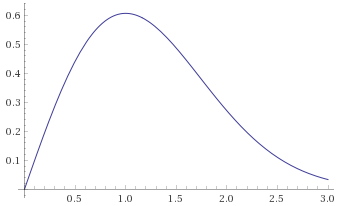
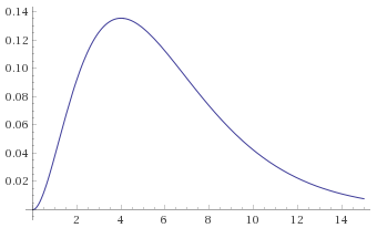
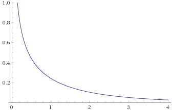
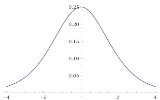
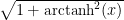
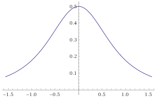
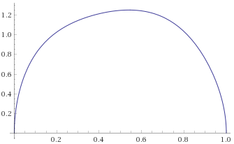
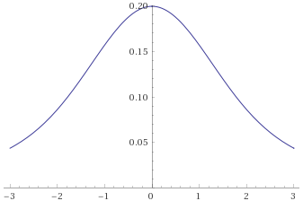
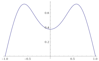
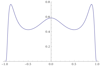
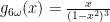
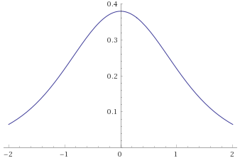
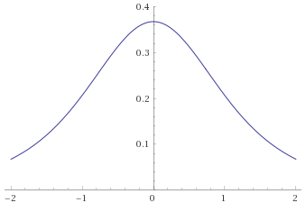
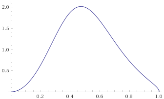
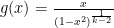
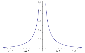
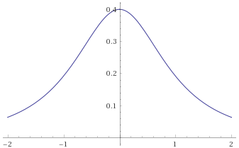
The trouble is, that everyone is so familiar with the Gaussian Distribution, that it is very seductive to shoehorn your data into it and try to use the familiar techniques to analyse your data. When people see a “bell curve”, their first thought is usually “looks like it is Gaussian distributed”, meaning that the data behaves like it has been sampled from the graph below:

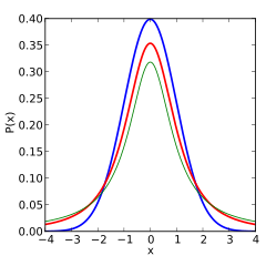
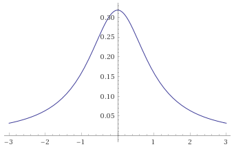
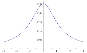
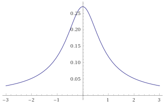
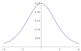
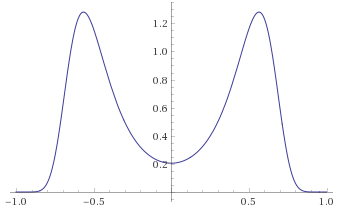
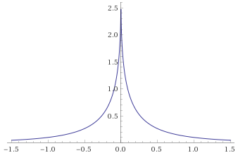
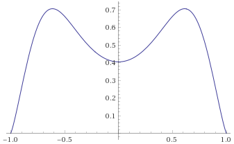
There are however many other distributions that are “bell curves”, and therefore look very similar to a Gaussian Distribution. Some of these behave very differently indeed when compared to the Gaussian Distribution, so it is important not to just default to using the Gaussian Distribution as soon as you see something that looks like a bell curve. By way of example, below are just two examples of distributions that are bell curves, but have very different behaviours to the Gaussian Distribution (in blue). The “Cauchy Distribution” is in green, and the “Students’s T Distribution with 2 degrees of freedom” is in red:

There is a fun bit of analysis that the data scientist Ethan Arsht did, comparing different military commanders throughout history to determine some sort of ranking for them, in a similar vein to baseball sabermetrics. To be clear – I like this analysis. It is a pretty neat insight, and took Ethan Arsht a lot of time and effort to put together, so I am not denigrating him or his conclusions in what I am about to say. It is just a perfect example of the kind of thing I am talking about, that lots of people do without really thinking about it (so, if you’re reading this Ethan, I apologise for using you as an example – there were probably lots of other examples I could have used).

In this article, he writes that the different commanders’ scores “largely adhere to a normal distribution”, and that Napoleon’s score is almost 23 standard deviations above the mean. The probability of an event occurring that is at least 22 standard deviations above the mean whilst being Gaussian Distributed is $\small 1.4 \times 10^{-107}$ . This is an incredibly minute number. For perspective, there have been around $\small 4 \times 10^{20}$ milliseconds since the big bang, and there are around $\small 3 \times 10^{80}$ particles in the observable universe. This means that if every single particle in the universe represented a new military commander every single millisecond since the big bang, we would only have seen $\small 1.2 \times 10^{101}$ military commanders so far, making it close to a 1 in a million chance that we would have encountered a single Napoleon in the entire history of this bizarre hypothetical universe of short-lived commander-particles.

The point of all of this, is that if you get an event that is almost 23 standard deviations above the mean assuming a Gaussian Distribution, then your data is NOT Gaussian Distributed. Even if you get an event “only” 6 standard deviations above (or below) the mean, this has a probability of around 1 in a billion, so unless you have an enormous amount of data already, it is pretty reasonable to suggest that your data isn’t as well behaved as a Gaussian Distribution would be. There is a good post on Slatestarcodex (still available in this archive) on conceptualising very small probabilities, which is useful for gaining a bit of intuition on the matter. Effectively, if the data was truly Gaussian Distributed, the outcome above is so vanishingly unlikely that it becomes more likely that you have either made a mistake in the analysis, or are simply hallucinating the whole thing.

II. Portioning

The most important way in which these other distributions differ from the Gaussian Distribution is how “heavy” their “tails” are. This basically means how quickly or slowly the probability declines as you move out to the far right or left of the distribution, and should be fairly easy to pick out on the graph above. If a distribution has heavier tails than a Gaussian Distribution, then more extreme events are more likely. Importantly, this is not the same as variance – a Gaussian Distribution with a high variance might permit a wide range of events with a reasonable probability, but an event that is 6 standard deviations above the mean is still around 1 in a billion. A heavy tailed distribution could be constructed to have the same variance, but such an event would be significantly more likely – perhaps 1 in 1000.

A useful concept to get across the idea of heavy tails is referred to as “portioning”. People’s heights can be considered to be roughly Gaussian distributed (we can ignore the fact that sexual dimorphism makes the distribution of heights bimodal, as this doesn’t significantly impact the tails). If someone selects two people at random from a population, add their heights together, and that sum is all that they tell you, you can make an educated guess about what you expect the individuals’ heights to be. If the sum is unusually large, say 400cm, you know that 200cm people are quite rare – around 1 in 1000, so picking 2 of them would be 1 in a million. On the other hand, whilst it could be an average height person at 175cm and an extremely tall person at 225cm, people that tall are more like 1 in 100 million, so given that the sum you were given is 400cm, unlikely though that result was, it is much more likely that the people measured were both very tall, around 200cm each, than it is that they managed to measure one of the vanishingly few people that is around 225cm tall. This is described as “even portioning”.

Wealth however is distributed according to a heavier tailed distribution – if you did the same thing but with people’s wealth rather than their height, and were given the sum of [/latex]1 billion, it would be possible for it to be two people each with wealth around [/latex]500 million each, but each of these is 1 in 300,000 making the probability of picking 2 of them 1 in 90 billion. Picking a person worth around [/latex]1 billion would be around 1 in 600,000 making it far more likely that the people were 1 average person and 1 billionaire, given the sum that you were told. This is described as the “concentrated portioning” – the majority of the sum is concentrated into one of the portions making up the sum. This concentrated portioning is a feature of heavier tails, and can generate useful intuitions about heavier tailed randomness. If you add more people/samples to the sum, the portioning may even out, with several samples contributing significantly to the sum – this is referred to as having concentrated short-run portioning but having even long-run portioning. If the tails are even heavier though, one sample could still dominate, contributing most of the sum’s value, no matter how many samples are summed together – this is referred to as concentrated long-run portioning.

III. Tail Terminology

Along the road to generating a structure from which to better perceive these concepts, there is some existing terminology that needs discussing, if only to immediately ignore it in favour of something better (seriously, feel free to skip to the next section).

Heavy tails technically means any tail that decays more slowly than that of the Exponential Distribution (it is defined in slightly more complicated and rigorous terms involving it’s “moment generating function” $\small M_x(t)=\int_{-\infty}^{\infty}{e^{tx}dF(x)=\infty\ \forall t>0}$ , but decaying slower than the Exponential Distribution is basically the end result). The Exponential Distribution is itself slightly heavier tailed than the Gaussian Distribution, but it is still fairly well behaved – it exhibits short-run concentration, but is even in the long-run.

Long tails are defined slightly differently, being distributions that obey the following formula: $\small \lim_{x\to\infty}\frac{P[X>x+t]}{P[X>x]}=1$ . This means that if the sample surpasses some high value, the probability approaches 1 that it will surpass any other higher value as the initial high value approaches infinity, or put more simply – “big events are likely to be even bigger”. This results in the vast majority of heavy tailed distributions also being long tailed, but it is technically possible for a distribution to be heavy tailed without being long tailed, if you contrive to make it irregular enough.

Sub-exponential tails are defined differently again, being distributions satisfying the formula: $\small \lim_{x\to\infty}\frac{P[X_1+X_2\leq x]}{P[X\leq x]}=2$ , for $\small X_1$ and $\small X_2$ being independent and identically distributed. This actually turns out to be an equivalent statement to having concentrated short-run portioning in the case where N=2 (the shortest possible run). Again, the vast majority of long tailed distributions are also sub-exponential, but it is technically possible to construct a long tailed distribution that is not sub-exponential.

We now have three terms that are almost equivalent to each other, but not quite. This is not useful for generating any kind of helpful structure, and it is not too surprising that heavy tails and long tails are used fairly interchangeably in most contexts. Aside from highly contrived distributions that are constructed solely to prove that the different definitions are not entirely equivalent, all commonly used distributions that are members of one of these sets are members of the other two sets as well. As being heavy tailed is the most inclusive set, I have chosen to use this terminology, but we ideally need something more informative.

One final term that can be used is fat tails. This is sometimes used to mean a tail that decays like (or slower than) a power law, such as a Pareto Distribution. This would make it refer to a significantly heavier tail than many sub-exponential distributions, and could potentially be a useful classification if it could be used unambiguously. Unfortunately, it is also often used synonymously with heavy tails, which removes any useful disambiguation properties it could have had.

IV. Mandelbrot’s Seven States of Randomness

Thankfully Benoit Mandelbrot developed a system of classification for types of randomness that allows us to classify different types of heavy tails much more reliably. It is still not particularly widely known about, but recent efforts by Nassim Taleb have spread the concept slightly beyond the academic community. The main issue with the classification system as a conceptual structure is that it is not particularly easy to visualise, and requires a relatively deep understanding of probability and mathematical terminology to work with. Mandelbrot started with 3 states – Mild, in which short-run portioning was even; Slow, in which short-run portioning was concentrated but long-run portioning became even; and Wild, in which long-run portioning remained concentrated. He then expanded upon this and in his book “Fractals and Scaling in Finance” Chapter E5, section 4.4, Mandelbrot lists “Seven States of Randomness”, which I have paraphrased below:

Proper Mild Randomness
- Short-run Portioning is even for N=2
Borderline Mild Randomness
- Short-run Portioning is concentrated
- Long-run Portioning becomes even, for some finite N
- The n^th root of the n^th moment grows like n
Delocalised Slow Randomness
- The n^th root of the n^th moment grows like a power of n
Localised Slow Randomness
- The n^th root of the n^th moment grows faster than any power of n
- All moments still finite
Pre-wild Randomness
- Moments grow so fast that some higher moments are infinite
- The 2^nd moment (variance) is still finite
- Long-run Portioning still becomes even, for a large enough finite N
Wild Randomness
- Even the 2^nd moment is infinite, so the variance is not defined
- There exists some moment (possibly fractional) $\small \mu_w,\ w>0$ that is still finite
- Long-run Portioning is concentrated for all N
Extreme Randomness
- All moments $\small \mu_w,\ w>0$ are infinite

The first couple of these make sense, given our understanding of portioning, but then they start being defined in relation to moments, so before moving on, let’s take pause to understand what this is saying (or skip to the next section, if you want to see a more intuitive approach). As a side-note, it is worth mentioning that “Delocalised” and “Localised” also refer to properties of moments of functions in these classes, however it will not be necessary to delve into the reasons behind this terminology, as other ways of defining these categories may be much more straightforward.

Firstly, the area under a distribution’s Probability Density Function is always 1 by necessity. The x-axis covers every possible eventuality, therefore the probability of an event occurring that is anywhere on the x-axis is a certainty. This means that for any Probability Density Function $\small f(x)$ , we have the identity $\small \int_{-\infty}^{\infty}{f(x)dx=1}$ , which can be referred to as the 0^th moment.

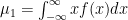
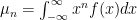
The mean of a distribution is calculated with the formula $\small \mu_1=\int_{-\infty}^{\infty}xf(x)dx$ and is known as the first moment, whilst the variance $\small \sigma^2=\mu_2 - \mu_1^2$ is the second central moment, closely related to the second moment $\small \mu_2=\int_{-\infty}^{\infty}{x^2f(x)dx}$ . More generally the nth moment is defined as $\small \mu_n=\int_{-\infty}^{\infty}{x^nf(x)dx}$ , and we can extend the concept to fractional n where this formula is still well defined.

This is the starting point for Mandelbrot’s definition of the later States of Randomness – if we create a new function based on these moments, giving us the x^th root of the x^th moment: $\small M(x)={(\mu_x)}^\frac{1}{x}$ , we can investigate how rapidly it grows, and compare it with other well known functions such as $\small x^n$ or $\small e^x$ .

The way to reliably compare functions in this way, is to look at their behaviour as x tends to infinity. If 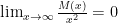$\small \lim_{x\to\infty}{\frac{M(x)}{x^2}}=0$ , we can say that $\small M(x)$ grows slower than $\small x^2$ , whilst if $\small \lim_{x\rightarrow\infty}{\frac{M(x)}{x^2}}=\infty$ , we can say that $\small M(x)$ grows faster than $\small x^2$ . In the eventuality that $\small 0<\lim_{x\rightarrow\infty}{\frac{M(x)}{x^2}}<\infty$ , we say that $\small M(x)$ grows like $\small x^2$ , regardless of what finite value the limit takes – simply multiplying or dividing $\small M(x)$ by a constant can make this limit equal to 1, meaning that the two functions are tending towards each other, which equates to them growing at the same rate.

Usefully, Mandelbrot has established that the growth rate of this function maps directly to the rate of decay of the right-hand tail of their corresponding Complimentary Cumulative Distribution Function (or Survival Function). Given a random variable X’s Probability Density Function $\small \phi(x)$ , its Cumulative Distribution Function is given by:

$\small \Phi(x)=P(X<x)=\int_{-\infty}^x \phi(t)dt$

Its Survival Function is then:

$\small S(x)=P(X>x)=1-\Phi(x)=\int_x^\infty \phi(t)dt$

Mandelbrot’s insight is the following:

If $\small {(\mu_x)}^\frac{1}{x}$ grows like $\small x^1$ , as per Borderline Mild Randomness, this is equivalent to the Survival Function $\small S(x)$ decaying like $\small e^{-x}$ , therefore the Exponential Distribution is necessarily a Borderline Mild distribution.
If $\small {(\mu_x)}^\frac{1}{x}$ grows like $\small x^n$ for some $\small n>1$ , as per Delocalised Slow Randomness, this is equivalent to the Survival Function decaying like $\small e^{-(x^{1/m})}$ for some $\small m>1$ . This is a family of functions that decay more slowly than $\small e^{-x}$ .
If $\small {(\mu_x)}^\frac{1}{x}$ grows faster than $\small x^n$ for any value of n but remains finite for $\small n<\infty$ , as per Localised Slow Randomness, this is equivalent to the Survival Function decaying like $\small e^{-({\ln (x)}^m)}$ for some $\small m>1$ . This family of functions decays slower still.
If $\small {(\mu_x)}^\frac{1}{x}$ is finite for $\small x=2$ , but grows so quickly that it becomes infinite for some finite value of x, as per Pre-Wild Randomness, this is equivalent to the Survival Function decaying like $\small x^{-\alpha}$ for some $\small \alpha>2$ . This means that the tails of the Probability Density Function $\small \phi(x)$ will decay like $\small x^{-(\alpha+1)}$ . Notably, the previous state’s decay rate of $\small e^{-({\ln (x)}^m)}$ stipulated that $\small m>1$ , because when we allow $\small m=1$ this simplifies to $\small e^{-({\ln (x)}^1)}=x^{-1}$ . As long as $\small m>1$ , this family of functions decays faster than a power law, whereas a Pre-Wild distribution’s Survival Function’s tail will decay as a power law (where the power is greater than 2).
By allowing for the second moment to become infinite as well, Wild Randomness is the domain of distributions whose Survival Function’s tails decay like $\small x^{-\alpha}$ and whose Probability Density Function’s tails decay like $\small x^{-(\alpha+1)}$ for $\small \alpha\le2$ .
Mandelbrot writes that Extreme Randomness is something that he “never encountered in practice”. The fact that such a distribution would not even have fractional moments is equivalent to the statement that its Survival Function decays slower than any power law, even fractional powers. This means that it must decay logarithmically.

After all of that, it is still difficult to gain an intuition about these states. The heuristic of even and concentrated portioning provides a basis for the original 3 states of Mild, Slow and Wild, but even then, if you are given the formula for a distribution, it is not obvious how you might go about classifying it. My aim is to come up with a way to more easily visualise how each of these classes of distributions behaves. Importantly, what I am doing below is not going to be a mathematical proof – it may well be provable, and the methodology below may suggest an approach, but I am only seeking to expound a heuristic here.

V. Compression

Given a particular distribution, it would be useful to be able to apply a transform to it that would bring the tails that disappear off towards infinity into a finite realm where they can be inspected. The idea here is to effectively “compress” the tails of the distribution into a finite interval in some sort of consistent way so that different distributions can be compared. Firstly, to keep things consistent and straightforward I will only use distributions that are either defined over the domain $\small (0,\infty)$ , or that are symmetric about 0 and defined over the domain $\small (-\infty,\infty)$ . The next thing to do is to ensure that the area under this new compressed curve is still 1, as was the case with the distribution itself beforehand.

One way to do this, is to find a function $\small g(x)$ that maps between the interval $\small (-\infty,\infty)$ and a finite interval. The hyperbolic tangent (or tanh) is one such function, mapping from $\small (-\infty,\infty)$ to $\small (-1,1)$ , however ideally we want a function the other way around, that takes in values from -1 to 1, and can output any real number. For this, we can simply use the hyperbolic tangent’s inverse function, referred to as $\small \textrm{arctanh}(x)$ or $\small \tanh^{-1}(x)$ .

Because the output of $\small \textrm{arctanh}(x)$ is a number in the interval $\small (-\infty,\infty)$ , we can feed this number into our probability density function $\small f(x)$ . These two functions combined are then $\small f(g(x))$ so if $\small g(x)=\textrm{arctanh}(x)$ , this give us $\small f(\textrm{arctanh}{(x)})$ . This is a transformed version of the probability density function fitting within $\small (-1,1)$ on the x-axis – very close to what we wanted. Below is a plot of the Gaussian Distribution (with mean 0 and variance 1) transformed in such a way:

This looks like it is doing what we want, but there is a little housekeeping left to do.

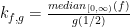
Firstly, we don’t want distributions with the same tail properties but different scales to behave differently under this transformation. For instance, this transform would look different if we used a Gaussian Distribution with variance 2 rather than 1, even though the choice of variance doesn’t change the tail behaviour. This also cannot be dealt with by simply adjusting for the variance of the distribution, as distributions classed as “Wild” do not have a well-defined variance. We can however use the median of right-handed distributions, and the third quartile of symmetric distributions. Keeping zero mapping to zero, we can map the median of a right handed distribution defined on $\small x\in[0,\infty)$ to 0.5, and we can map the third quartile of a distribution symmetric about 0 to 0.5 (effectively mapping to 0.5 the median of the part of the distribution defined on $\small [0,\infty)$ , which keeps both types consistent). This means that we want to adjust the transformation to make $\small g(0.5)={median}_{[x,\infty)}(f)$ , which would then neatly split the transformed graph into 4 vertical sections of equal width $\small (-1,-0.5),\ (-0.5,0),\ (0,0.5),\ (0.5,1)$ corresponding to the intervals on the untransformed distribution of the four quartiles (or above and below the median for right-handed distributions). For $\small g(x)=\textrm{arctanh}(x)$ , we find that $\small \textrm{arctanh}{(0.5)}=\frac{log(3)}{2}$ so we can simply rearrange this equation to give $\small \frac{2}{\log(3)}\textrm{arctanh}{(0.5)}=1$ . This suggests that we should use $\small g(x)={median}_{[0,\infty)}(f)\frac{2}{\log(3)}\textrm{arctanh}{(x)}$ going forwards, or for a more general function $\small g(x)$ , we want to look at the transformation $\small f(g(x)\times\frac{{median}_{[0,\infty)}(f)}{g(1/2)})$ .

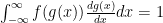
Secondly, the area under this graph is clearly not 1, so we need to adjust the transformation to make it preserve the area. This turns out to be very easily doable by an application of the chain rule – we know that $\small \int_{-\infty}^{\infty}{f(x)dx=1}$ , and for any function $\small g(x)$ , the chain rule gives us $\small \int_{-\infty}^{\infty}{f(g(x))\frac{dg(x)}{dx}dx=1}$ . This means that our transformation simply needs to be multiplied by the derivative of $\small g(x)\times\frac{{median}_{[0,\infty)}(f)}{g(1/2)}$ , and it will meet our requirements. The expression $\small k_{f,g}=\frac{{median}_{[0,\infty)}(f)}{g(1/2)}$ is a constant with respect to x, and can therefore be taken outside the derivative if necessary, so if we refer to this transformation as $\small T_g(f,x)$ , we get:

$\small T_g(f,x)=f(k_{f,g}\ g(x))k_{f,g}\frac{dg(x)}{dx},\ where\ g(x)=\textrm{arctanh}(x),\ \ k_{f,g}=\frac{{median}_{[0,\infty)}(f)}{g(1/2)}$

$\small T_g(f,x)=\frac{2{\ median}_{[0,\infty)}(f)}{log(3)}\frac{1}{1-x^2}f(\frac{2\ {median}_{[0,\infty)}(f)}{\log{(3)}}\textrm{arctanh}{(x)})$

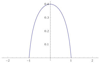
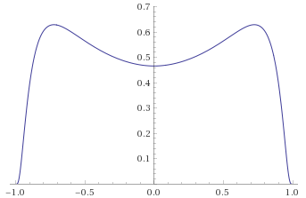
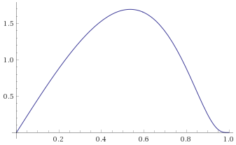
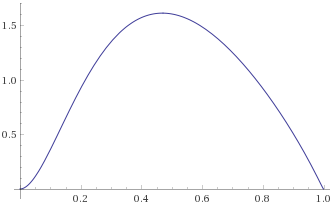
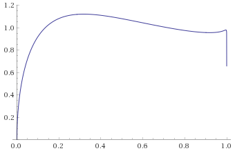
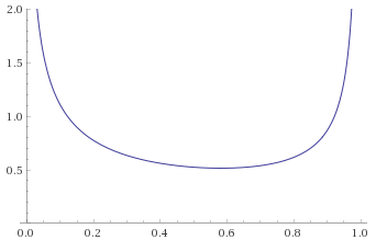
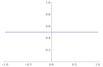
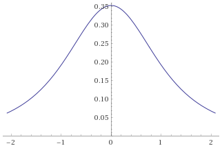
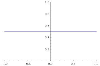
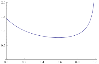
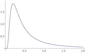
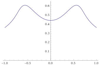
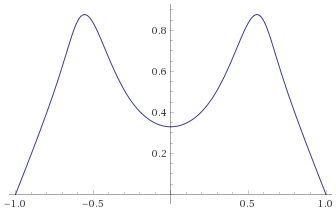
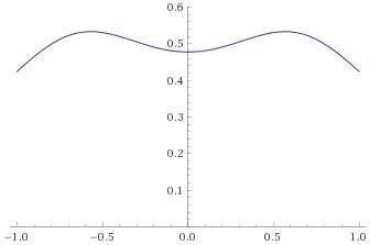
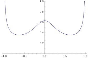
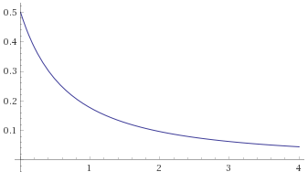
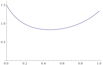
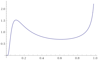
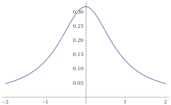
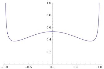
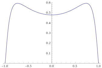
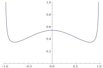
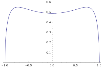
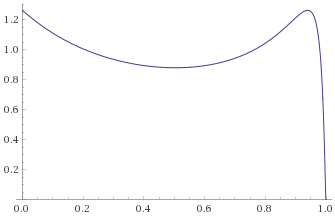
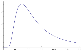
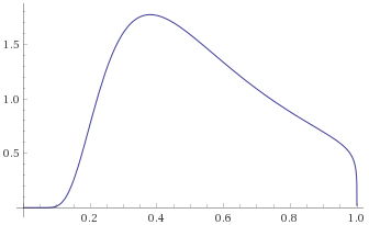
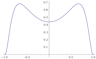
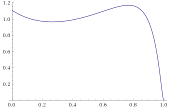
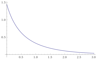
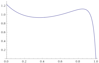
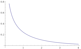
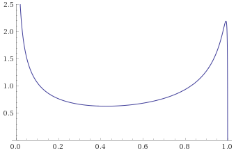
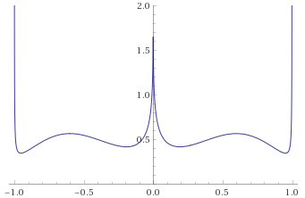
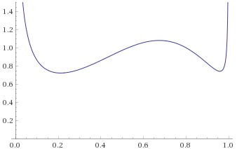
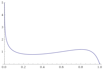
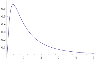
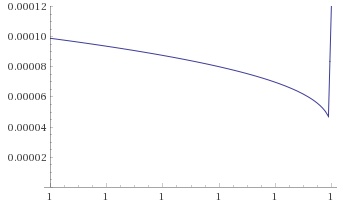
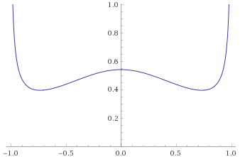
This is still a very easy to apply transformation and we can see how it treats the Gaussian Distribution now that it has been adjusted to renormalize horizontal scaling and preserve the area under the curve.

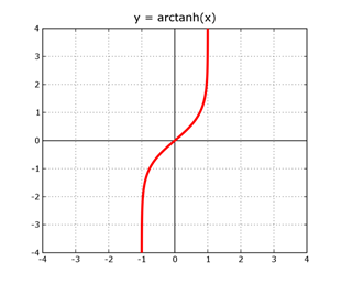
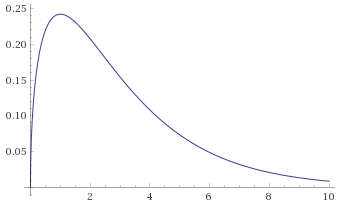
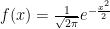
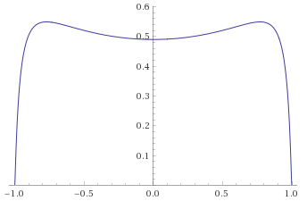
The Gaussian Distribution (mean 0, variance 1), given by the probability density function $\small f(x)=\frac{1}{\sqrt{2\pi}}e^{-\frac{x^2}{2}}$ is shown on the two graphs below, before and after transformation:

You can easily reproduce the second plot by typing the following into Wolfram Alpha, noting that the Gaussian Distribution with mean 0 and variance 1 has its third quartile at 0.67449 so you have 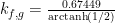$\small k_{f,g}=\frac{0.67449}{\textrm{arctanh}(1/2)}$ :

plot 1/sqrt(2π) e^(-g^2/2) dg/dx substitute g=0.67449 arctanh(x)/arctanh(0.5) from x=-1..1 y=0..0.6

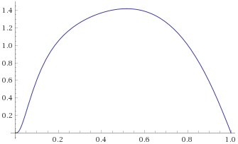
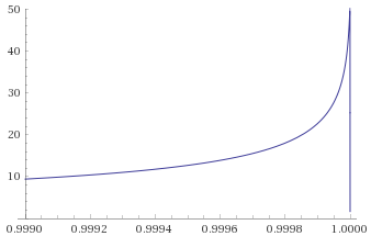
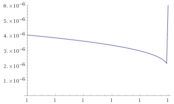
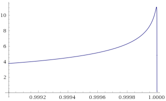
Importantly, this function is still 0 at x=1 and x=-1. Furthermore, as the area under the graph has been preserved by the transformation, the area under the curve between say x=0.99 and x=1 is the same as the area under the original un-transformed probability density function between $\small x=\frac{2\times0.67449}{\log(3)}\textrm{arctanh}(0.99)=3.25$ and $\small x=\infty$ , or more generally $\small \int_{t}^{1}{T_g(f,x)dx}=\int_{k_{f,g}\ g(t)}^{\infty}f(x)dx$ . It can also be verified that using a Gaussian Distribution with a different variance gives the same result (e.g. variance of 4, which results in a third quartile at 1.34898).

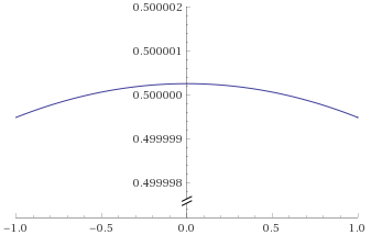
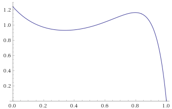
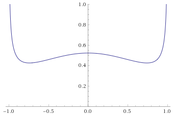
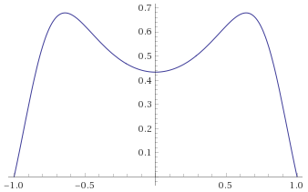
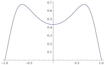
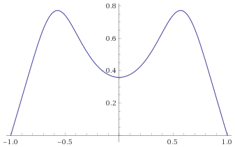
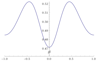
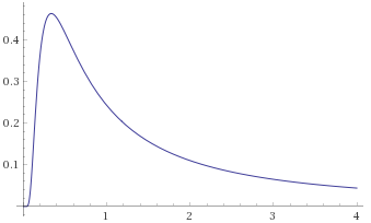
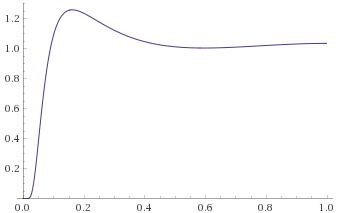
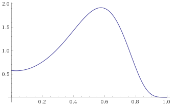
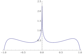
In terms of Mandelbrot’s seven states, the Gaussian Distribution falls into the Mild class. The transformation’s behaviour at $\small \pm1$ is fundamentally a statement about the tails, and the fact that they go to 0 under this transformation tells us that they decay at a certain rate. Whilst not yet a mathematically rigorous concept, it is easy to see how other distributions whose transformations also go to 0 at $\small \pm1$ might decay at similar enough rates to be counted as Mild. Let’s look at how this transformation treats a few different distributions.

Generalised Gaussian Distribution with shape parameter 3 [before, after] – this distribution has even lighter tails than the Gaussian Distribution, which is reflected in the way that the “shoulders” of the second graph fall towards zero earlier than they did for the Gaussian Distribution:

Maxwell Distribution (also known as the Chi Distribution with 3 degrees of freedom) [before, after]:

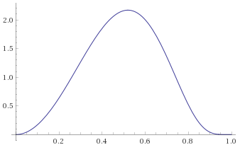
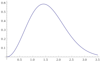
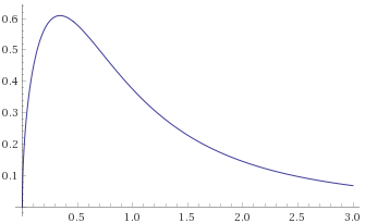
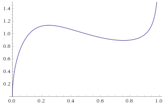
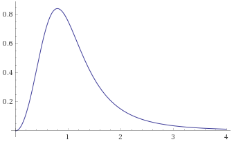
Rayleigh Distribution with scale parameter 1 (also known as the Chi Distribution with 2 degrees of freedom) [before, after] – note again that a different scale parameter results in the same transformed graph – the Rayleigh Distribution with scale parameter $\small 1/\sqrt2$ (also known as the Weibull Distribution with shape parameter 2) has different mean and variance, but the transformation maps it to the same shape:

Chi-Squared Distribution with 6 degrees of freedom (also known as the Gamma Distribution with shape parameter 3 and scale parameter 2) [before, after] – again, a Gamma Distribution with shape parameter 3 and scale parameter 1/3 is mapped to the same shape:

Chi-Squared Distribution with 3 degrees of freedom (also known as the Gamma Distribution with shape parameter 1.5 and scale parameter 2) [before, after]:

All of the above distributions are in the Mild category, and conveniently all go to zero at $\small x=1$ (even the last one – it is just such a steep curve that Wolfram Alpha doesn’t plot it).

VI. The Borderline

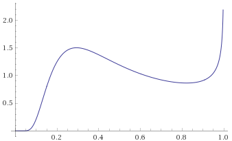
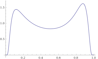
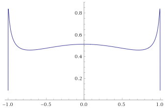
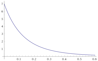
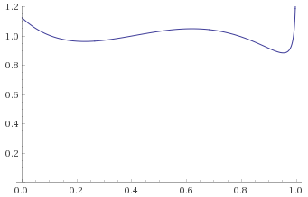
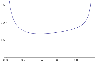
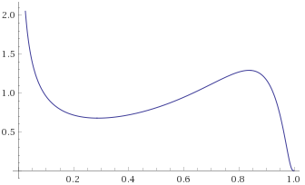
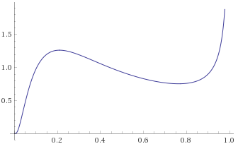
What happens when we try a few Borderline Mild distributions?

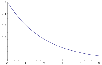
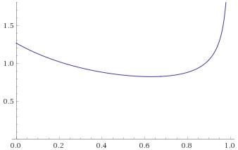
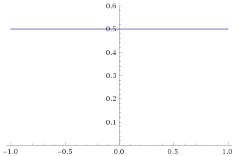
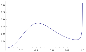
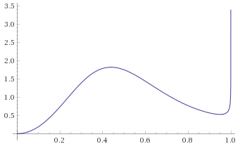
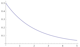
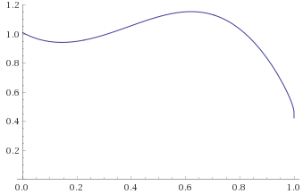
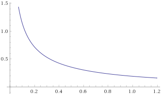
Exponential Distribution, scale ½ (also Gamma Distribution, shape 1, scale 2; Weibull Distribution, shape 1 scale 2; Chi Squared Distribution, 2 degrees of freedom) [before, after]:

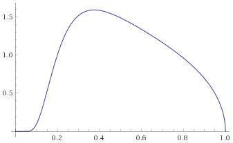
Chi-Squared Distribution, 1 degree of freedom (also Gamma Distribution, shape 0.5, scale 2) [before, after]:

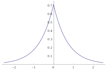
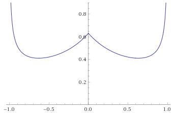
Laplace Distribution (also known as Generalised Gaussian Distribution with shape parameter 1) [before, after] – this distribution is a scaled exponential distribution reflected about the y-axis:

Logistic Distribution [before, after]:

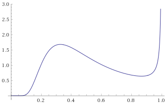
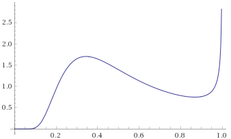
None of these distributions go to zero at $\small x=1$ , which is again very convenient. Their curves either go to some finite value or shoot off to infinity as x tends towards 1. As a heuristic, this gives us a good measure for when something is Mild – if this transformation goes to zero at $\small x=1$ , it is Mild, otherwise it is Borderline Mild or worse. As an aside, this transformation for the Logistic Distribution is interesting because it is a straight line. This is a direct consequence of the fact that the cumulative distribution function for the Logistic Distribution is itself a scaled hyperbolic tangent function $\small \frac{1}{2}+\frac{1}{2}\tanh(\frac{x}{2s})$ where s is the scale parameter. We can prove that this is in fact exactly a straight line as follows:

$\small T_g(f,x)=f(k_{f,g}\ g(x))k_{f,g}\frac{dg(x)}{dx},\ where\ k_{f,g}=\frac{{median}_{[0,\infty)}(f)}{g(1/2)}$

$\small Substitute\ g(x)=\textrm{arctanh}(x),\ g(1/2)=\frac{\log(3)}{2}$

$\small T_g(f,x)=\frac{2\ {median}_{[0,\infty)}(f)}{\log(3)}\frac{1}{1-x^2}f(\frac{2\ {median}_{[0,\infty)}(f)}{\log(3)}\textrm{arctanh}(x))$

$\small Substitute\ f(x)=\frac{1}{4s}\sinh^2(\frac{x}{2s}),\ {median}_{[0,\infty)}(f)=s\log(3)$

$\small T_g(f,x)=\frac{2s\log(3)}{log(3)}\frac{1}{1-x^2}\frac{1}{4s}\textrm{sech}^2\left(\frac{\frac{2s\log(3)}{\log(3)}\textrm{arctanh}(x)}{2s}\right)$

$\small T_g(f,x)=\frac{1}{1-x^2}\frac{1}{2}\textrm{sech}^2(\textrm{arctanh}(x))$

$\small T_g(f,x)=\frac{1}{1-x^2}\frac{1}{2}(\sqrt{1-x^2})^2$

$\small T_g(f,x)=\frac{1}{2}\ (for\ x\neq\pm1)$

Going forwards, as shorthand I shall refer to a transformation taking a distribution to zero at $\small x=1$ as the transformation having “tamed” the distribution. As the above transformations have not tamed these Borderline Mild distributions, they are not going to tame any distributions that are in a higher state of randomness either. The question therefore is, how do we tell the difference between all the other states of randomness?

VII. Transformation Family

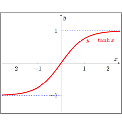
The function we have used so far $\small g(x)=\textrm{arctanh}(x)$ is only one of many inverse-sigmoid curves that would serve a similar purpose of compressing the domain $\small (-\infty,\infty)$ down to $\small (-1,1)$ . We can construct a whole range of different transformations for different functions $\small g(x)$ that are of the form:

$\small T_g(f,x)=f(k_{f,g}\ g(x))k_{f,g}\frac{dg(x)}{dx},\ where\ k_{f,g}=\frac{{median}_{[0,\infty)}(f)}{g(1/2)}$

The most fundamental properties that $\small g(x)$ must have, are that it is continuous, monotonically increasing, asymptotic at $\small x=\pm1$ , and that $\small g(x)=-g(-x)$ . Beyond this though, if we are looking to discern different tail behaviours, we need different functions $\small g(x)$ that are asymptotic at different speeds. For a function that tends to infinity at $\small x=1$ , $\small \textrm{arctanh}(x)$ tends to infinity exceedingly slowly. Putting some numbers in, we get $\small \textrm{arctanh}(0.99)=2.65$ , $\small \textrm{arctanh}(0.9999)=4.95$ , $\small \textrm{arctanh}(0.999999)=7.25$ . Every time we get 100 times closer to 1, we still only go up by around 2, so in order to compress the tails of heavier tailed distributions more, what we need is a function that gets there faster.

We can construct a faster growing function by multiplying $\small g(x)$ by a function that is symmetric about the origin and increases as it gets closer to $\small \pm1$ . We don’t need to worry too much about what values it actually takes as long as it is positive and non-zero, as the transformation uses $\small k_{f,g}$ to ensure that it will scale the whole thing appropriately, mapping $\small g(1/2)$ to the value that is the median of the positive half of the distribution. Let’s start with $\small 1+x^2$ , as the slowest growing symmetrical polynomial:

$\small {T_g(f,x)=f(k_{f,g}\ g(x))k_{f,g}\frac{dg(x)}{dx},\ where\ g(x)=(1+x^2)\textrm{arctanh}(x),\ \ k_{f,g}=\frac{{median}_{[0,\infty)}(f)}{g(1/2)}}$

We can of course multiply it by this again and again, building up a whole family of transformations, each growing faster than the last:

$\small g_0(x)=\textrm{arctanh}(x)$

$\small g_1(x)=(1+x^2)\textrm{arctanh}(x)$

$\small g_2(x)=(1+x^2)^2\textrm{arctanh}(x)$

$\small g_3(x)=(1+x^2)^3\textrm{arctanh}(x)$

$\small \vdots$

$\small g_n(x)=(1+x^2)^n\textrm{arctanh}(x)$

But there is still further that we can go; $\small (1+x^2)^n$ is not asymptotic, so the function $\small \textrm{arctanh}(x)$ grows faster than it. We can make something symmetric and non-zero by taking $\small \sqrt{1+\textrm{arctanh}^2(x)}$ . We can therefore multiply $\small g_0(x)$ by this to get another family of transformations, again each growing faster than the last, with the first one ultimately growing faster than any in the previous list:

$\small g_{\omega+1}(x)=\sqrt{1+\textrm{arctanh}^2(x)}\textrm{arctanh}(x)$

$\small g_{\omega+2}(x)=(1+\textrm{arctanh}^2(x))\textrm{arctanh}(x)$

$\small g_{\omega+3}(x)=(1+\textrm{arctanh}^2(x))^\frac{3}{2}\textrm{arctanh}(x)$

$\small g_{\omega+4}(x)=(1+\textrm{arctanh}^2(x))^2\textrm{arctanh}(x)$

$\small \vdots$

$\small g_{\omega+n}(x)=(1+\textrm{arctanh}^2(x))^\frac{n}{2}\textrm{arctanh}(x)$

This is still not the fastest $\small g(x)$ we can find though – the reciprocal of any polynomial will grow faster than any power of $\small arctanh(x)$ , so we can take the non-zero symmetric function $\small \frac{1}{\sqrt{1-x^2}}$ and multiply it by x to get another inverse-sigmoid curve that grows faster than any of the above, then keep multiplying it by the symmetric function for another list (please excuse the slightly odd choice of subscripts – it is done to avoid confusion later):

$\small g_{2\omega-2}(x)=\frac{x}{\sqrt{1-x^2}}$

$\small g_{2\omega}(x)=\frac{x}{1-x^2}$

$\small g_{3\omega}(x)=\frac{x}{(1-x^2)^\frac{3}{2}}$

$\small g_{4\omega}(x)=\frac{x}{(1-x^2)^2}$

$\small \vdots$

$\small g_{n\omega}(x)=\frac{x}{(1-x^2)^\frac{n}{2}}$

Finally, we can construct yet another that will grow faster than any of these (it would of course be possible to construct yet faster ones, but this will suffice for our purposes here):

$\small g_{\omega^2}(x)=\sinh(\frac{x}{1-x^2})$

Armed with this array of transformations, we can return to looking at some more heavy tailed distributions.

VIII. The Wilderness

In his book “Fractals and Scaling in Finance”, Mandelbrot mentions that the Slow states of randomness (Borderline Mild, Slow Delocalised, Slow Localised and Pre-Wild) are more subtle to deal with, and I quite agree. As such, I shall start looking at the Wild states first. To remind ourselves; Wild Randomness occurs when even the 2nd moment is infinite, so the variance is not defined. There exists some moment (possibly fractional) $\small \mu_w,\ w>0$ that is still finite, and Long-run Portioning is concentrated for all N.

In fact, I am inclined to draw a further distinction between the states of randomness for which Long-run Portioning is concentrated for all N (those being Wild and Extreme according to Mandelbrot). The Wild category as defined by Mandelbrot has a natural dividing line at the point where the 1st moment ceases to be defined – splitting the category into those distributions with a mean, and those whose mean is also undefined. It is undeniable that a distribution whose mean is undefined is significantly more pathological than one which has a mean, so it makes sense to split these out. If you are sampling from a distribution whose mean is undefined and you try to take the mean of your sample, you can calculate it, but as you take more samples the sample mean you are calculating will never converge to a value – the samples you take will occasionally be so vast that it will shift the mean significantly in a random direction, no matter how many samples you have already taken.

If we continue to refer to the state of randomness with undefined variance but valid mean as Wild Randomness, we can refer to the state with undefined mean but some valid fractional moment as Aggressively Wild randomness, or perhaps Aggressive randomness for short. It is worth noting that this Aggressive state is different from the Extreme state, for which not even fractional moments exist. I have seen it written or implied occasionally that the Extreme category includes anything which has an undefined 1st moment, but this is incorrect as per Mandelbrot’s original framing of the states.

When he says that he never encountered Extreme randomness in practice, he wasn’t forgetting things like the Cauchy Distribution and the Lévy Distribution, both of which are relatively well known distributions with an undefined mean. Unlike genuinely Extreme randomness however, they do have fractional moments, for example the $\small \frac{1}{4}^{th}$ moment of the Lévy Distribution is $\small \int_0^\infty x^{\frac{1}{4}} \frac{1}{\sqrt{2\pi}} \frac{e^{-\frac{1}{2x}}}{x^\frac{3}{2}}dx\approx 1.72$ . I shall refer to this category as Aggressive, to set them apart from both the Wild and the Extreme, but make no mistake – the state of Extreme randomness really is not inappropriately named – by not even having fractional moments that are defined, no matter how tiny, they really are teetering on the boundary of being valid probability distributions at all.

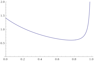
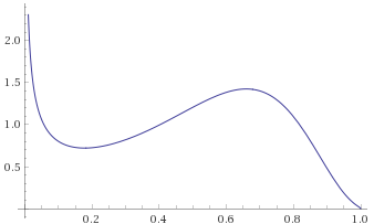
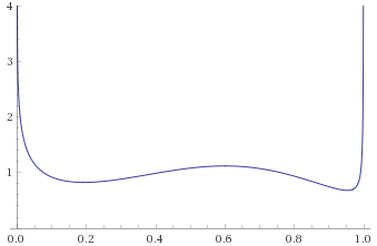
Initially, let’s restrict ourselves to the Wild category (by which I mean not the Aggressive category). To start with, let’s see what happens when we use $\small g_{2\omega-2}(x)=\frac{x}{\sqrt{1-x^2}}$ and $\small g_{2\omega}(x)=\frac{x}{1-x^2}$ for our transformation – we can apply these to a few different distributions to get the idea.

Student’s T Distribution, 2 degrees of freedom [before, transform 1, transform 2]:

Arcsinh-Logistic Distribution, shape parameter 2 (this is the distribution of a random variable, the inverse hyperbolic sine of which is distributed like a Logistic Distribution with scale parameter 2) [before, transform 1, transform 2]:

Pareto Distribution, shape parameter 2 [before, transform 1, transform 2]:

Fisk Distribution, shape parameter 1.5 (also Log-Logistic Distribution shape 1.5 – this is the distribution of a random variable, the logarithm of which is distributed like a Logistic Distribution with scale parameter 1.5) [before, transform 1, transform 2]:

Inverse-Chi-Squared Distribution, 3 degrees of freedom (also Inverse-Gamma Distribution, shape 1.5, scale 0.5) [before, transform 1, transform 2]:

We can see from all of these, that the $\small g_{2\omega-2}(x)=\frac{x}{\sqrt{1-x^2}}$ transformation does not tame them, but $\small g_{2\omega}(x)=\frac{x}{1-x^2}$ does.

IX. Getting More Aggressive

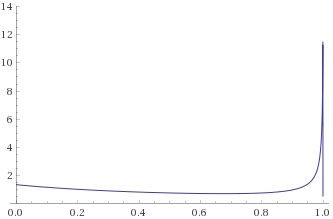
We can now see whether the state of Aggressive randomness behaves differently (spoilers – it does). Let’s use $\small g_{2\omega}(x)=\frac{x}{1-x^2}$ and $\small g_{4\omega}(x)=\frac{x}{(1-x^2)^2}$ to assess these, and where neither of them successfully tame the distribution, we can try $\small g_{\omega^2}(x)=\textrm{sinh}(\frac{x}{1-x^2})$ as well.

Slash Distribution [before, transform 1, transform 2]:

Cauchy Distribution (also Student’s T Distribution, 1 degree of freedom; Stable Distribution, stability parameter 1, skewness parameter 0) [before, transform 1, transform 2]:

Arcsinh-Logistic Distribution, shape parameter 1 [before, transform 1, transform 2]:

Student’s T Distribution, 0.5 degrees of freedom [before, transform 1, transform 2, transform 3]:

Pareto Distribution, shape parameter 1 (also Fisk Distribution, shape 1; Log-Logistic Distribution, shape 1) [before, transform 1, transform 2]:

Lévy Distribution (also Inverse-Chi-Squared Distribution, 1 degree of freedom; Inverse-Gamma Distribution, shape 0.5, scale 0.5; Stable Distribution, stability parameter 0.5, skewness parameter 1) [before, transform 1, transform 2, transform 3]:

We can see that 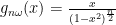$\small g_{2\omega}(x)=\frac{x}{1-x^2}$ no longer tames these distributions, but $\small g_{4\omega}(x)=\frac{x}{(1-x^2)^2}$ tames some of them, and $\small g_{\omega^2}(x)=\textrm{sinh}(\frac{x}{1-x^2})$ tames them all. In fact, for any distribution in this category, there should be some $\small g_{n\omega}(x)=\frac{x}{(1-x^2)^\frac{n}{2}}$ that does the job. We can observe that a distribution resembling a power law with an exponent k will be tamed by $\small g(x)=\frac{x}{{(1-x^2)}^\frac{k}{k-1}}$ , for example the Pareto Distribution with shape parameter 0.5 has a term like $\small \frac{1}{x^{1.5}}$ and is tamed by $\small g_{6\omega}(x)=\frac{x}{(1-x^2)^3}$ as $\small \frac{1.5}{0.5}=3$ . As the exponent k in a power law can be arbitrarily close to 1, the power required to tame an Aggressive distribution could be arbitrarily high. This is fine though, as because $\small g_{\omega^2}(x)=\textrm{sinh}(\frac{x}{1-x^2})$ grows faster than all of them, it should tame any distribution that is aggressive.

Now we just need to make sure that Extreme distributions behave yet differently, to make sure that we can tell the difference using these transformations. We can use $\small g_{\omega^2}(x)=\textrm{sinh}(\frac{x}{1-x^2})$ again, to see what happens.

Arcsinh-Cauchy Distribution (this is the distribution of a random variable, the inverse hyperbolic sine of which is distributed like a Cauchy Distribution) [before, after]:

Log-Cauchy Distribution (this is the distribution of a random variable, the logarithm of which is distributed like a Cauchy Distribution) [before, after]:

Unlike the Aggressive distributions, these Extreme distributions are not tamed by this transformation, which is useful as it allows us to distinguish between the different categories.

X. The Liquids of Randomness

We have now picked the low hanging fruit. Rather poetically, Mandelbrot likens the states of randomness to the states of matter – Solid, Liquid and Gas compared with Mild, Slow and Wild. Mild randomness behaves metaphorically like a solid – unsurprising and inert – the extremes in your data/model won’t really be extreme at all. Wild randomness (encompassing Wild, Aggressive and Extreme) behaves like a gas – all over the place, but obeying its own rules that make sense – extremes are the defining feature of your data/model. Slow randomness (encompassing Borderline Mild, Slow Delocalised, Slow Localised and Pre-Wild) he compares with a liquid – a strange mixture of both behaviours, sometimes acting in ways that a solid might (falling from a height, water is as unforgiving as concrete/with enough data, you find that the extremes are effectively bounded), but other times behaving similar to a gas (liquids get everywhere/with a small enough sample, the extremes dominate enough to skew the data). It is clear from this, that Mandelbrot considers Slow randomness to be tricky to deal with.

We have already established the boundaries of Slow randomness (again – heuristically, not by proof). We know that $\small g_0(x)=\textrm{arctanh}(x)$ is insufficient to tame Borderline Mild distributions, and by virtue of Wild distributions being tamed by $\small g_{2\omega}(x)=\frac{x}{1-x^2}$ but not by $\small g_{2\omega-2}(x)=\frac{x}{\sqrt{1-x^2}}$ , we can assume that Pre-Wild distributions will be tamed by $\small g_{2\omega-2}(x)=\frac{x}{\sqrt{1-x^2}}$ . This means that anything that is not tamed by $\small g_0(x)=\textrm{arctanh}(x)$ , but is tamed by $\small g_{2\omega-2}(x)=\frac{x}{\sqrt{1-x^2}}$ should be Slow randomness, but that spans four of Mandelbrot’s states, so it would be useful if we could be more specific.

Thankfully, in between these two functions, we have already established that there are a couple of families of functions that may be instructive: $\small g_n(x)=(1+x^2)^n\textrm{arctanh}(x)$ and $\small g_{\omega+n}(x)=(1+\textrm{arctanh}^2(x))^\frac{n}{2}\textrm{arctanh}(x)$ . In fact, we can eke out a third (which will hopefully slightly justify the slightly contrived choice of subscript earlier), by noting that we can take the third family $\small g_{n\omega}(x)=\frac{x}{(1-x^2)^\frac{n}{2}}$ and extend it in the other direction, starting with $\small g_{2\omega-2}(x)=\frac{x}{\sqrt{1-x^2}}$ :

$\small g_{2\omega-2}(x)=\frac{x}{\sqrt{1-x^2}}$

$\small g_{2\omega-3}(x)=\frac{x}{\sqrt[3]{1-x^2}}$

$\small g_{2\omega-4}(x)=\frac{x}{\sqrt[4]{1-x^2}}$

$\small \vdots$

$\small g_{2\omega-n}(x)=\frac{x}{\sqrt[n]{1-x^2}}$

No matter how large n becomes, there will be a point after which $\small g_{2\omega-n}(x)$ starts to grow faster than $\small g_{\omega+n}(x)$ . These three families are exactly what we need, but the words “there will be a point after which” already indicate where the problem lies. We can construct transformations that might theoretically discern between the types of slow randomness, but the behaviour that we are interested in (what happens at $\small x=1$ ) may cease to be obvious. Let’s try anyway and see what goes wrong.

Having just dealt with the Wild category, we can start with the distributions exhibiting Pre-Wild randomness. Many of these look like power laws, similar to the Wild distributions that were tamed by $\small g_{2\omega}(x)=\frac{x}{1-x^2}$ , so the obvious thing to try is $\small g_{2\omega-2}(x)=\frac{x}{\sqrt{1-x^2}}$ and $\small g_{2\omega-n}(x)=\frac{x}{\sqrt[n]{1-x^2}}$ . For simplicity, we can use $\small g_{2\omega-8}(x)=\frac{x}{\sqrt[8]{1-x^2}}$ , $\small g_{2\omega-4}(x)=\frac{x}{\sqrt[4]{1-x^2}}$ and $\small g_{2\omega-2}(x)=\frac{x}{\sqrt{1-x^2}}$ :

Student’s T Distribution, 5 degrees of freedom [before, transform 1, transform 2, transform 3]:

Student’s T Distribution, 3 degrees of freedom [before, transform 1, transform 2, transform 3]:

Pareto Distribution, shape 7 [before, transform 1, transform 2, transform 3]:

Fisk Distribution, shape 3 (also Log-Logistic Distribution, shape 3) [before, transform 1, transform 2, transform 3]:

Inverse-Chi-Squared Distribution, 5 degrees of freedom (also Inverse-Gamma Distribution, shape 2.5, scale 0.5) [before, transform 1, transform 2, transform 3]:

In a similar manner to the Aggressive category, we can suggest a fairly sensible rule of thumb. It looks like a Probability Density Function that behaves like $\small \frac{1}{x^{k}}$ (which implies a Survival Function that behaves like $\small \frac{1}{x^{k-1}}$ ) will be tamed by $\small g(x)=\frac{x}{{(1-x^2)}^\frac{1}{k-2}}$ , for example the Pareto Distribution with shape parameter 10 has a term like $\small \frac{1}{x^{11}}$ and is tamed by $\small g_{2\omega-9}(x)=\frac{x}{\sqrt[9]{1-x^2}}$ . This appears to be related to the largest moment that is defined for these distributions – for a distribution whose Probability Density Function resembles a power law with exponent k, the largest moment that is defined will be $\small \mu_{k-2}$ (again, for example, the Student’s T Distribution with 4 degrees of freedom has a Probability Density Function that behaves like $\small \frac{1}{x^5}$ and has a defined skewness ( $\small \mu_3$ ) but undefined kurtosis ( $\small \mu_4$ ), fitting this trend).

The issue with this, is that although we have that a Pre-Wild distribution will be tamed by $\small g_{2\omega-2}(x)=\frac{x}{\sqrt{1-x^2}}$ , and there will be some n for which it is not tamed by $\small g_{2\omega-n}(x)=\frac{x}{\sqrt[n]{1-x^2}}$ , this n could be arbitrarily large. We cannot exhaustively search through to find the n at which the transformation ceases to tame the distribution. Therefore, unless we come across one that does fail to tame it, we can’t be sure that the distribution isn’t in a different category of Slow randomness.

Skipping to the other end of the spectrum of Slow randomness, we can look at distributions that we know are Borderline Mild (the same ones as in the borderline section). We can hypothesise that they will be tamed by $\small g_n(x)=(1+x^2)^n\textrm{arctanh}(x)$ for some n (and therefore that $\small g_{\omega+1}(x)=\sqrt{1+\textrm{arctanh}^2(x)}\textrm{arctanh}(x)$ will tame all of them as well). We can apply $\small g_1(x)=(1+x^2)\textrm{arctanh}(x)$ , $\small g_8(x)=(1+x^2)^8\textrm{arctanh}(x)$ and $\small g_{\omega+1}(x)=\sqrt{1+\textrm{arctanh}^2(x)}\textrm{arctanh}(x)$ to see the effect:

Logistic Distribution [before, transform 1, transform 2, transform 3]:

Exponential Distribution [before, transform 1, transform 2, transform 3]:

Exponential-Logarithmic Distribution, shape 0.5, scale 1 [before, transform 1, transform 2, transform 3]:

Chi-Squared Distribution with 1 degree of freedom [before, transform 1, transform 2, transform 3]:

With the Chi-Squared Distribution with 1 degree of freedom, it becomes apparent what the problem is. As per Mandelbrot, all Gamma Distributions with shape parameter $\small \le1$ are Borderline Mild, so if the hypothesis is correct, we will still need higher and higher powers of $\small (1+x^2)$ to tame the function as the shape parameter gets smaller. There is no limit to how high this power might need to be. The effect of $\small g_{\omega+1}(x)$ however is equally unhelpful – we can see that as the shape parameter gets smaller, even though it is always zero at $\small x=1$ , it can spike arbitrarily high just before 1, giving the illusion that it is not going to zero after all.

We can similarly hypothesise that Slow Delocalised randomness is tamed by $\small g_{\omega+n}(x)=(1+\textrm{arctanh}^2(x))^\frac{n}{2}\textrm{arctanh}(x)$ for some n, but this has similar problems. We can apply $\small g_8(x)=(1+x^2)^8\textrm{arctanh}(x)$ and $\small g_{\omega+4}(x)=(1+\textrm{arctanh}^2(x))^2\textrm{arctanh}(x)$ to see:

Generalised Gaussian Distribution, shape ½ [before, transform 1, transform 2]:

Generalised Gaussian Distribution, shape ¼ [before, transform 1, transform 2]:

Weibull Distribution, shape ½ [before, transform 1, transform 2]:

Generalised Exponential Distribution, shape ¼ [before, transform 1, transform 2]:

Here we have the opposite problem – distributions that look like they are going to zero under $\small g_8(x)$ , but that actually shoot off to infinity at the last moment – a problem that gets worse with $\small g_n(x)$ as n increases. Clearly, even if these two hypotheses are true, it is not necessarily reliable for easily distinguishing between Borderline Mild and Slow Delocalised, as the behaviour at $\small x=1-\epsilon$ may not be indicative of whether the transformation goes to zero at $\small x=1$ or not.

We are left with the Slow Localised category, which is epitomised by the Lognormal Distribution. The Lognormal is very commonly used in a lot of analysis, because its straightforward relation to the Gaussian Distribution makes it very easy to work with. Mandelbrot however, really doesn’t like the Lognormal Distribution – in fact he devotes an entire chapter of his book to why its overuse is so problematic. He states:

“It is beloved because it passes as mild: moments are easy to calculate and it is easy to take for granted that they play the same role as for the Gaussian. But they do not. They hide the difficulties due to skewness and long-tailedness behind limits that are overly sensitive and overly slowly attained”

“This distribution should be avoided. A major reason… is that a near-lognormal’s population moments are overly sensitive to departures from exact lognormalities. A second major reason… is that the sample moments are not to be trusted, because the sequential sample moments oscillate with sample size in erratic and unmanageable manner.”

It is this category then, that we are left with, having no easy families of transformations left to try. These distributions should have tails that are eventually heavier than any Slow Delocalised distribution, but lighter than any Pre-Wild distribution. This means, that if the above heuristics are correct, they should not be tamed by any transformation using $\small g_{\omega+n}(x)=(1+\textrm{arctanh}^2(x))^\frac{n}{2}\textrm{arctanh}(x)$ , but should be tamed by every transformation using $\small g_{2\omega-n}(x)=\frac{x}{\sqrt[n]{1-x^2}}$ .

Of course, the issues we established with the Borderline Mild and Slow Delocalised distributions are very much relevant here. The heuristic may have been somewhat informative for the other categories of Slow randomness – allowing positive identification of many distributions that don’t require us to delve too deeply into any of the infinite families of transformations, and whose transforms don’t have behaviour at $\small x=1-\epsilon$ that is too pathologically different to their behaviour at $\small x=1$ . Unfortunately, the Slow Localised category falls right into the middle of the gap between two of the infinite families of transformations, which renders the heuristic unable to determine whether the distribution is truly Slow Localised, or if it is just a particularly badly behaved Slow Delocalised or Pre-Wild distribution. In fact, if we try to use the transformations $\small g_{\omega+2}(x)=(1+\textrm{arctanh}^2(x))\textrm{arctanh}(x)$ and $\small g_{2\omega-4}(x)=\frac{x}{\sqrt[4]{1-x^2}}$ on a couple of Slow Localised distributions, we get very odd results. The additional two graphs show the same transforms, but zoomed in very close to $\small x=1$ :

Lognormal Distribution [before, transform 1, transform 2]:

Arcsinh-Gaussian Distribution [before, transform 1, transform 2]:

We can see that the graphs look the wrong way around – the distributions look like they are tamed by $\small g_{\omega+2}(x)$ , and not tamed by $\small g_{2\omega-4}(x)$ , which should not be possible. It is only when we zoom in incredibly far, that we see that the opposite is in fact true.

If we tried with transforms based on $\small g_{\omega+3}(x)$ or $\small g_{2\omega-5}(x)$ , this would only get worse – requiring zooming in even further (potentially further than is actually possible using Wolfram Alpha).

XI. Stability

Having trawled through all of the States of Randomness, it is worth noting a very important property of Wild, Aggressive and Extreme randomness – they no longer obey the classical Central Limit Theorem.

The Central Limit Theorem states that if you add n i.i.d (independent and identically distributed) random variables together, the sum of the variables will tend towards being distributed according to a Gaussian Distribution as $\small n\to\infty$ . This however only applys when these random variables are distributed according to a distribution with finite variance (which means either a Mild or a Slow distribution).

If you have i.i.d. random variables that are distributed according to a Probability Density Function with tails that decay like $\small x^{-\alpha-1}$ (or equivalently a Survival Function that decays like $\small x^{-\alpha}$ , also known as “Paretian Tails”), the Generalised Central Limit Theorem states that for $\small 0<\alpha\le2$ (Wild and Aggressive randomness), this sum will tend towards being distributed according to a “Stable Distribution” with “stability parameter” $\small \alpha$ .

These Stable Distributions have the same kind of Paretian tails as the distributions that generated them, so for example, the sum of n random variables that were generated by a Student’s T Distribution with 1.5 degrees of freedom will tend towards being distributed according to a Stable Distribution with stability parameter 1.5 as $\small n\to\infty$ . It is for this reason that Mandelbrot refers to Wild randomness as “Tail Preserving”.

The stability parameter that defines the family of Stable Distributions can vary between $\small 0<\alpha\le2$ , and the Stable Distribution with stability parameter 2 is the Gaussian Distribution. This has several implications:

Pre-Wild randomness (Paretian tails with $\small \alpha>2$ ) falls under the classical Central Limit Theorem, so under these conditions all will tend towards the Stable Distribution with stability parameter 2 (the Gaussian Distribution)
Wild randomness with $\small \alpha=2$ (e.g. Student’s T Distribution with 2 degrees of freedom, Fisk Distribution with shape parameter 2, Pareto Distribution with shape parameter 2 and Inverse-Chi-Squared distribution with 4 degrees of freedom) will actually still tend towards the Gaussian Distribution in this limit, however for any finite sum of n random variables, the sum’s distribution will still have undefined variance.
Wild randomness with $\small 1<\alpha<2$ and Aggressive randomness $\small 0<\alpha\le1$ will tend towards a non-Gaussian, heavy tailed Stable Distribution with stability parameter $\small =\alpha$ in this limit.
Extreme randomness is still not covered by this theorem, as Extreme distributions have tails that are even heavier than Paretian tails. These are rarely used distributions, but it does not appear to be known what their behaviour is in this limit.

Most Stable Distributions have Probability Density Functions that are not expressable in terms of elementary functions, which makes them rather hard to deal with (with the exception of the Gaussian, Cauchy and Levy distributions). Their stability under summation of random variables was a key feature that Mandelbrot was interested in however, due to his focus on fractals and self-similarity. If you have a stochastic process whose evolution over time is self-similar (for instance its movements over a day are indistinguishable from its movements over a year), which he hypothesised was the case for the stock market and commodity prices, you have a situation where the sum of multiple random variables (daily movements) must behave the same as the individual random variables themselves (minute by minute movements). In other words, random variables distributed according to a Stable Distribution.

XII. Conclusion

At this point, it is natural to ask what has been achieved by all of this. The claims above are not rigorously proven, therefore the transformation discussed is only a heuristic. Hopefully however, it provides a useful lens with which to view the tail behaviour of various distributions, giving more of an intuitive feel of how different heavy behave.

Whilst Mandelbrot’s book originates the concept, it is first and foremost an academic text from someone at the forefront of a field of study, which makes it unsurprisingly dense and impenetrable. It provides the basis for the taxonomy he developed, but is remarkably short on examples, which are often a good way to gain understanding of a topic. He did write another book aimed at a more general audience, that is much more accessible and gets across some of his ideas in this area. I highly recommend reading it, but unfortunately one thing that it doesn’t go into much detail on, is this taxonomy for classifying randomness.

Dealing with heavy tails is an area of probability that is hugely important for understanding real-world processes, and the tendency for people to try to shoe-horn their data into Gaussian or Lognormal models is likely due to the underdevelopment of tools for dealing with these other types of randomness. As such, I hope that the plethora of examples above is able to make the concepts slightly more accessible and encourage further exploration.

In summary, assuming that the behaviour of the transformation $\small T_g(f,x)=f(k_{f,g}\ g(x))k_{f,g}\frac{dg(x)}{dx},\ where\ k_{f,g}=\frac{{median}_{[0,\infty)}(f)}{g(1/2)}$ is as described, we can add it to the descriptions of the different states of randomness that were listed earlier. This gives us the following:

Proper Mild Randomness
- Short-run Portioning is even for N=2
- $\small T_g(f,1)=0$ for $\small g(x)=\textrm{arctanh}(x)$
Borderline Mild Randomness
- Short-run Portioning is concentrated
- Long-run Portioning becomes even, for some finite N
- The n^th root of the n^th moment grows like n
- Right-hand tail of the Survival Function decays like $\small e^{-x}$
- $\small T_g(f,1)\neq0$ for $\small g(x)=\textrm{arctanh}(x)$
- $\small T_g(f,1)=0$ for $\small g(x)=(1+x^2)^n\textrm{arctanh}(x)$ for some $\small n>0$
Delocalised Slow Randomness
- The n^th root of the n^th moment grows like a power of n
- Right-hand tail of the Survival Function decays like $\small e^{-(x^{1/m})}$ for some $\small m>1$
- $\small T_g(f,1)\neq0$ for $\small g(x)=(1+x^2)^n\textrm{arctanh}(x)$ for all n>0
- $\small T_g(f,1)=0$ for $\small g(x)=(1+\textrm{arctanh}^2(x))^\frac{n}{2}\textrm{arctanh}(x)$ for some $\small n>0$
Localised Slow Randomness
- The n^th root of the n^th moment grows faster than any power of n
- All moments still finite
- Right-hand tail of the Survival Function decays like $\small e^{-({\ln(x)}^m)}$ for some $\small m>1$
- (In principle, $\small T_g(f,1)\neq0$ for $\small g(x)=(1+\textrm{arctanh}^2(x))^\frac{n}{2}\textrm{arctanh}(x)$ for all $\small n>0$ )
- (In principle, $\small T_g(f,1)=0$ for $\small g(x)=\frac{x}{\sqrt[n]{1-x^2}}$ for all $\small n>1$ )
Pre-wild Randomness
- Moments grow so fast that some higher moments are infinite
- The 2^nd moment (variance) is still finite
- Long-run Portioning still becomes even, for a large enough finite N
- Right-hand tail of the Survival Function decays like $\small x^{-\alpha}$ for some $\small \alpha>2$
- $\small T_g(f,1)\neq0$ for $\small g(x)=\frac{x}{\sqrt[n]{1-x^2}}$ for some $\small n>2$
- $\small T_g(f,1)=0$ for $\small g(x)=\frac{x}{\sqrt{1-x^2}}$
Wild Randomness
- Even the 2^nd moment is infinite, so the variance is not defined
- The 1st moment (mean) is still finite
- Long-run Portioning is concentrated for all N
- Right-hand tail of the Survival Function decays like $\small x^{-\alpha}$ for some $\small 1<\alpha\le2$
- $\small T_g(f,1)\neq0$ for $\small g(x)=\frac{x}{\sqrt{1-x^2}}$
- $\small T_g(f,1)=0$ for $\small g(x)=\frac{x}{1-x^2}$
Aggressive Randomness
- Even the 1^st moment is undefined There exists some moment (possibly fractional) $\small \mu_w,\ w>0$ that is still finite
- Right-hand tail of the Survival Function decays like $\small x^{-\alpha}$ for some $\small 0<\alpha\le1$
- $\small T_g(f,1)\neq0$ for $\small g(x)=\frac{x}{1-x^2}$
- $\small T_g(f,1)=0$ for $\small g(x)=\textrm{sinh}(\frac{x}{1-x^2})$
Extreme Randomness
- All moments $\small \mu_w,\ w>0$ are infinite
- $\small T_g(f,1)\neq0$ for $\small g(x)=\textrm{sinh}(\frac{x}{1-x^2})$