Bayesian Updating

By Mellivora | 4 April 2020 | Comments 0 Comments
Epistemic Status: 4/4 - Maximum Effort

Sections:
Question
Preparation
Solution
Verification
Generalisation
Extension

Question

You have a randomly biased coin picked from the uniform distribution U(0,1). It is flipped 3 times and comes up heads twice and tails once. What is probability that 4^th flip is a head?

This is a question that we can answer using Bayesian Updating, but unlike most simple examples of Bayes Theorem, we are not updating a single probability but an entire probability distribution. There are many very good explanations of how to apply Bayes Theorem to update a single probability (video, article). The principle is the same for updating a distribution, but it is a little more involved.

Preparation

To make this more intuitive, we can imagine a joke shop with a vending machine for biased coins: we pull a lever, and it dispenses a coin, but we don’t know what its bias is. We know that it could be biased anything from always heads to always tails, and anything in between, and we presume that the machine is stocked with an equal number of coins of any particular bias.

Therefore, when we pick up the coin the machine has dispensed, we know that it has a particular bias, that won’t change, but we don’t know what that bias is. For all we know, it could be an unbiased coin, coming up heads 50% of the time, but it could just as easily be one that is biased to come up heads 75% of the time, or 1% of the time, and all we know is what we get when it is flipped. Intuitively, we can see that these flips do provide us with some information, because if we flipped the coin thousands of times and it came up heads around 2/3 of the time, we would be able to be fairly confident that it had a bias towards heads of around 2/3. The question is about how much just 3 flips tell us. Importantly, the question is not asking us to determine the exact bias of the coin, or even the most likely bias of the coin, but just the probability of a head given the information that we know.

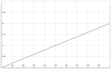
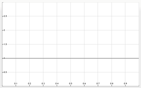
The Prior Distribution for the coin’s bias towards heads is $\small f_0 (x)=U(0,1)$ shown below – the x-axis represents the coin’s bias towards heads (0 being always tails, 1 being always heads), and the y-axis represents likelihood of coin having that bias, so every bias starts out equally likely. As with any probability distribution, the total area underneath the curve will be 1, and for this scenario the curve is 0 everywhere else, as a coin cannot be heads 110% of the time.

The area under the graph between two points ∆x apart on the x-axis represents the probability of the coin’s bias being between those two values e.g. $\small P(0.3 \leq Bias<0.4)= \int_{0.3}^{0.4} f_0 (x)dx= \frac{1}{10}$ , so 1/10 of the coins produced by the machine will have a bias towards heads between 0.3 and 0.4. We could treat this range as a hypothesis, and perform Bayesian Updating using the techniques in the links above to determine how likely this hypothesis is given the evidence (this calculation is included below for completeness):

$\small P(Hypothesis|Evidence)=\frac{P(Evidence|Hypothesis)P(Hypothesis)}{P(Evidence)}$

$\small P(0.3\le Bias<0.4|2\ Heads\ in\ 3\ flips)=\frac{P(2\ Heads\ in\ 3\ flips|0.3\le Bias<0.4)P(0.3\le Bias<0.4)}{P(2\ Heads\ in\ 3\ flips)}$

$\small =\frac{\frac{3\int_{0.3}^{0.4}{(1-x)x^2 f_0 (x) dx}}{\int_{0.3}^{0.4}{f_0 (x) dx}}\int_{0.3}^{0.4}{f_0 (x) dx}}{3\int_{0}^{1}{(1-x)x^2 f_0 (x) dx}}=\frac{3\int_{0.3}^{0.4}{(1-x)x^2 \cdot 1dx}}{3\int_{0}^{1}{(1-x)x^2 \cdot 1dx}}=\frac{3\left[\frac{1}{3}x^3-\frac{1}{4}x^4\right]_{0.3}^{0.4}}{3\left[\frac{1}{3}x^3-\frac{1}{4}x^4\right]_0^1}$

$\small =\frac{\frac{3}{3}{0.4}^3-\frac{3}{4}{0.4}^4-\frac{3}{3}{0.3}^3-\frac{3}{4}{0.3}^4}{\frac{3}{3}-\frac{3}{4}-0}=\frac{\frac{2560-768-1080+243}{40000}}{\frac{1}{4}}=\frac{191}{2000}=9.55\%$

This is fine, but only gives us a single number – the probability that the bias is between 0.3 and 0.4 given the evidence of 2 heads and a tail. What we want is the entire probability distribution given the evidence, known as the Posterior Distribution. We could divide the whole x-axis into tenths, and do the above process multiple times over for each possible hypothesis – $\small H_1:0\le Bias<0.1,\ H_2:0.1\le Bias<0.2,\ etc.$ , however this would still only give us an approximation to the Posterior Distribution. We need to take this idea, and reduce the size of the intervals on the x-axis, in order to increase the resolution.

$\small P(H_n|E)=\frac{P(E|H_n)P(H_n)}{\sum_{i}{P(E|H_i)P(H_i)}}$

In the limit as ∆x→0 we get the exact Posterior Distribution, however there is a slight problem – if ∆x is zero, the area of a vertical strip ∆x wide is also zero, so both $\small P(H_n|E)=0$ and $\small P(H_n)=0$ which is not very helpful. Instead of doing this straight away then, before we take this limit we can replace the two offending terms with approximations that will become accurate in the limit. Our Prior Distribution is $\small f_0(x)$ and if we call the Posterior Distribution $\small f_1(x)$ we have:

$\small P(H_n)\approx f_0(x)\Delta x\ where\ x=average\ bias\ under\ H_n$

$\small P(H_n|E)\approx f_1(x)\Delta x\ where\ x=average\ bias\ under\ H_n$

We then have:

$\small f_1(x)\Delta x\approx\frac{P(E|H_n)f_0(x)\Delta x}{\sum_{i}{P(E|H_i)P(H_i)}}$

We can then cancel out the ∆x on both sides, before taking the limit as ∆x→0 which renders the approximation accurate and turns the sum into an integral, giving us:

$\small f_1(x)=\frac{P(E|H_n)f_0(x)}{\int_{0}^{1}{P(E|H_y)P(H_y)}}$

As above, $\small P(H_n)\approx f_0(x)\Delta x$ so in the limit as ∆x→0 we get $\small P(H_y)=f_0(y)dy$ , giving:

$\small f_1(x)=\frac{P(E|H_n)f_0(x)}{\int_{0}^{1}{P(E|H_y)f_0(y)dy}}$

With this groundwork done, we want to construct the Posterior Distribution for the coin’s bias. Here, the evidence is the result of the coin flips, and the hypotheses are the different biases that the coin may have, so we can restate the above formula like this:

$\small f_1(x)=\frac{P(Result|Bias=x)f_0(x)}{\int_{0}^{1}{P(Result|Bias=y)f_0(y)dy}}$

Thankfully, we are now rid of the word “Hypothesis”, so going forwards we can use H to refer to Heads without risking confusion.

Solution

Taking it one step at a time, we should be able to see the distribution change with each new coin flip. Let us assume that the coin tosses were H, H, T such that the first result is H, and calculate the first Posterior Distribution – the distribution of what we expect the coin’s bias to be, given that the first toss was H. The probability of a coin flip coming up Heads given that the coin has a bias x is simply x, therefore $\small P(Result=H|Bias=x)=x$ . We can substitute this straight into our formula:

$\small f_1(x)=\frac{xf_0(x)}{\int_{0}^{1}{{xf}_0(x)dx}}$

Of course, $\small f_0(x)=U(0,1)=1\ for\ 0\le x\le 1$ so this simplifies to:

$\small f_1(x)=\frac{x\cdot 1}{\int_{0}^{1}{x\cdot 1dx}}=\frac{x}{\left[\frac{1}{2}x^2\right]_0^1}=\frac{x}{\frac{1}{2}-0}=2x$

This gives us the Posterior Distribution $\small f_1(x)=2x$ which is shown below (of course, this only applies for $\small 0\le\ x\le 1$ and outside of this, the distribution is still 0):

We can do the same again, using the Posterior Distribution as our new Prior Distribution for the second flip, which again came up H:

$\small f_2(x)=\frac{xf_1(x)}{\int_{0}^{1}{xf_1(x)dx}}=\frac{x\cdot2x}{\int_{0}^{1}{x\cdot2xdx}}=\frac{2x^2}{\left[\frac{2}{3}x^3\right]_0^1}=\frac{2x^2}{\frac{2}{3}-0}=3x^2$

This gives us a new Posterior Distribution $\small f_2(x)=3x^2$ shown below:

The third flip comes up T, so our calculation needs to be slightly different. Because T happens whenever H does not happen, $\small P(T|Bias=x)=1-x$ . This gives us the following formula:

$\small f_3(x)=\frac{(1-x)f_2(x)}{\int_{0}^{1}{(1-x)f_2(x)dx}}=\frac{(1-x)\cdot3x^2}{\int_{0}^{1}{(1-x)\cdot3x^2dx}}=\frac{(1-x)\cdot3x^2}{\left[x^3-\frac{3}{4}x^4\right]_0^1}=\frac{(1-x)\cdot3x^2}{\frac{1}{4}-0}=12(1-x)x^2$

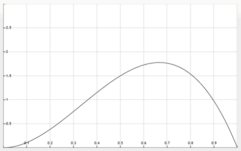
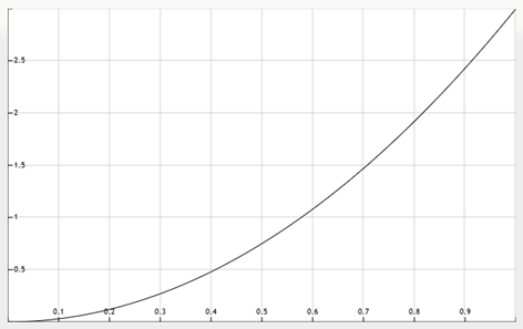
Finally, we have the Posterior Distribution after HHT 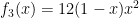$\small f_3(x)=12(1-x)x^2$ which is shown below:

On this graph, we can see some things that agree with our intuition about the question. Firstly, the probability of the bias being either 0 or 1 (all tails or all heads) is 0, because we have already seen both tails and heads come up. Secondly, the maximum on the graph is at 2/3 – this is the most likely bias for the coin, given that it has come up with 2 heads out of 3 flips. This is not the same however as saying that the probability of the 4^th flip being heads is 2/3 – this is only the most likely of many possible biases that the coin could have, and there is more area under the graph below 2/3 than above it, suggesting that the expected probability of the flip coming up heads should be less than 2/3. The graph of $\small f_2(x)=3x^2$ had a maximum at x=1, meaning that after the first two tosses, the most likely bias was “always heads”, but it is obviously incorrect to expect a coin to come up heads with probability 1 after simply witnessing it come up heads twice in a row.

What we need to do, in order to find the answer to the original question of what the probability is of the 4^th flip being a head, is to find the mean of this distribution. This is simply the sum of all possible biases x multiplied by the probability of the coin having that bias, for which we can use our new Posterior Distribution $\small f_3(x)$ :

$\small P(H|HHT)=\int_{0}^{1}{xf_3(x)dx}$

Substituting in $\small f_3(x)=12(1-x)x^2$ gives us:

$\small P(H|HHT)=\int_{0}^{1}{x\cdot12(1-x)x^2dx}=\left[{\frac{12}{4}x}^4-\frac{12}{5}x^5\right]_0^1=\frac{12}{4}-\frac{12}{5}-0=\frac{3}{5}$

Therefore, in fact the probability that the 4^th flip comes up heads is 60%

Verification

We can in fact skip straight from $\small f_0(x)$ to $\small f_3(x)$ in a single step. If we take the result to be 2 Heads in 3 flips, which given a bias of x towards heads has a probability of x (for the first head), times x (for the second head), times (1-x) for the tails, we have:

$\small P(Result=2\ Heads\ in\ 3\ flips|Bias=x)=P(2H\ in\ 3|x)=(1-x)x^2$

Which we can substitute in:

$\small f_3(x)=\frac{P(Result|Bias=x)f_0(x)}{\int_{0}^{1}{P(Result|Bias=y)f_0(y)dy}}$

$\small f_3(x)=\frac{P(2H\ in\ 3|x)f_0(x)}{\int_{0}^{1}{P(2H\ in\ 3|y)f_0(y)dy}}$

$\small f_3(x)=\frac{(1-x)x^2f_0(x)}{\int_{0}^{1}{(1-x)x^2f_0(x)dx}}$

$\small f_3(x)=\frac{(1-x)x^2\cdot1}{\int_{0}^{1}{(1-x)x^2\cdot1dx}}$

$\small f_3(x)=\frac{(1-x)x^2}{\left[\frac{1}{3}x^3-\frac{1}{4}x^4\right]_0^1}$

$\small f_3(x)=\frac{(1-x)x^2}{\frac{1}{12}-0}$

$\small f_3(x)=12(1-x)x^2$

Which is unsurprisingly the same Posterior Distribution and will therefore give the same answer that the next flip is 60% likely to come up heads, or $\small P(H|2H\ in\ 3)=60\%$ .

Using this Posterior Distribution, we can also find the probability that the coin is within a range of biases, like we did at the start:

$\small P(0.3\le Bias<0.4|2\ Heads\ in\ 3\ flips)=\int_{0.3}^{0.4}{12(1-x)x^2dx}=\left[\frac{12}{3}x^3-\frac{12}{4}x^4\right]_{0.3}^{0.4}$

$\small =4\cdot{0.4}^3-3\cdot{0.4}^4-4\cdot{0.3}^3+3\cdot{0.3}^4=\frac{2560-768-1080+243}{10000}=\frac{191}{2000}=9.55\%$

Again, unsurprisingly, this is the same result that we found by performing the calculation the other way.

As an aside, it is worth noting that in the first calculation of this probability; we made use of the observation that:

$\small P(2\ Heads\ in\ 3\ flips)=3\int_{0}^{1}{(1-x)x^2f_0(x)dx}=3\left[\frac{1}{3}x^3-\frac{1}{4}x^4\right]_0^1=\frac{1}{4}$

The 3 before the integral is there because there are 3 ways to get 2 heads in 3 flips – HHT, HTH and THH, which must be summed over. This result is interesting however, because although on the first flip of a new, completely unknown coin, the probability of getting H is 50% (the same as for an unbiased coin), the probability of getting 2 heads in the first 3 flips is only 25%, whereas if we knew that the coin was unbiased, the probability would be 37.5% or 3/8. It can equivalently be shown that the fact that the bias of the coin is random with uniform distribution rather than being unbiased makes the probability of getting 3 heads in a row 25% as well, rather than the 12.5% we would expect from normal coins.

Generalisation

This result can be generalised to n coin flips, of which k are heads:

$\small f_{n,k}(x)=\frac{{(1-x)}^{n-k}x^kf_0(x)}{\int_{0}^{1}{{(1-x)}^{n-k}x^kf_0(x)dx}}$

Helpfully, there is an integral known as the Beta function that supplies an identity that allows us to simplify this.

$\small B(x,y)=\int_{0}^{1}{t^{x-1}{(1-t)}^{y-1}dt}=\frac{(x-1)!(y-1)!}{(x+y-1)!}$

Assuming it is still the case that $\small f_0(x)=U(0,1)$ , we can use the Beta function $\small B(k+1,n-k+1)$ to evaluate the integral, giving us:

$\small \int_{0}^{1}{{(1-x)}^{n-k}x^kdx=}\frac{(n-k)!k!}{(n+1)!}$

Which allows us to simplify $\small f_{n,k}(x)$ to:

$\small f_{n,k}(x)=\frac{(1-x)^{n-k}x^k}{\frac{(n-k)!k!}{(n+1)!}}=\frac{(n+1)!(1-x)^{n-k}x^k}{(n-k)!k!}$

Using this, we can find the probability that the next flip will come up heads after any number of flips, again using the formula for the mean of a distribution:

$\small P(H|k\ Heads\ in\ n\ flips)=\int_{0}^{1}{xf_{n,k}(x)dx}=\frac{(n+1)!}{(n-k)!k!}\int_{0}^{1}{(1-x)^{n-k}x^{k+1}dx}$

Now, using the Beta function $\small B(k+2,n-k+1)$ , this integral can be found to be:

$\small \int_{0}^{1}{(1-x)^{n-k}x^{k+1}dx}=\frac{(k+1)!(n-k)!}{(n+2)!}$

Therefore, we end up with the following:

$\small P(H|kH\ in\ n)=\frac{(n+1)!}{(n-k)!k!}\frac{(k+1)!(n-k)!}{(n+2)!}$

Most of which cancels out to leave:

$\small P(H|kH\ in\ n)=\frac{(k+1)}{(n+2)}$

This remarkably simple formula therefore allows us to quickly calculate:

$\small P(H|3H\ in\ 5)=\frac{4}{7}$

$\small P(H|4H\ in\ 7)=\frac{5}{9}$

$\small P(H|5H\ in\ 9)=\frac{6}{11}$

$\small P(H|17H\ in\ 100)=\frac{18}{102}=\frac{3}{17}$

This generalised result is actually far more useful than it first appears – it is not just applicable to coin flips, but to most processes that have a binary outcome. One that is highly relevant to everyday life is that of positive and negative reviews in online shopping – Grant Sanderson has a brilliant video about this on his channel 3Blue1Brown. If you haven’t already seen the video, I highly recommend it, as his videos are very effective at making seemingly counter-intuitive things understandable.

To cut a long story short though – online shopping reviews can be treated in exactly the same way as flipping a uniformly distributed biased coin – no further alteration is required. Let $\small P(G)$ be the probability that you have a good shopping experience with a retailer that has a certain number of positive and negative reviews:

$\small P(G|100\%\ with\ 5\ reviews)\equiv P(H|5H\ in\ 5)=\frac{6}{7}=85.7\%$

$\small P(G|90\%\ with\ 40\ reviews)\equiv P(H|36H\ in\ 40)=\frac{37}{42}=88.1\%$

Extension

Given a randomly biased die, it is rolled n times and you record the results, what can you say about its Posterior Distribution?

This is more difficult – what does it mean for the die to be randomly biased? Now there are 6 possible outcomes rather than 2, so we can’t just treat the distribution as a single dimensional graph where rolling 1 with probability p means that rolling 6 has probability (1-p) as we did with the coin, because each of the other numbers can have independent probabilities too. There are in fact 5 degrees of freedom – you have to know the probabilities of 5 of the faces of the biased die before you can calculate the 6^th. If you only know the probabilities of faces 1-4, and they don’t yet add up to 100% (say they add up to 80%), face 5 could still be anywhere between 0% and 20% with face 6 making up the remainder.

We don’t want to be messing around with 5-dimensional graphs, so what we can do is model the die as a sequence of biased coin flips. If instead of a single biased coin, we have 5 separate coins that are each flipped once in turn, to represent a single roll of the die, with each of the coins able to have its own independent bias, we should be able to make a working model of the die. When flipping the first coin, H represents 1 and T represents 2-6. If the flip comes up T, we flip the second coin, and H represents 2, with T representing 3-6. Whenever we get H we can stop, but each time T comes up, we flip the next coin to see if the die has rolled the next number until the 5^th coin in which T represents 6.

In this way we need 5 of the graphs – one for the bias of each hypothetical coin, in order to fully understand the biases of all of the faces of the die, but we can treat each graph separately. This also has the advantage of allowing us to use the formulae we derived for the coin. There is still a problem however – with the single coin, our Prior Distribution was given, however we don’t know what to use as a prior for each of the 5 new hypothetical coins. We can’t use the uniform distribution for the 1^st coin, as it has a mean of 0.5 – that would mean that given a randomly selected die, we would expect it to roll a 1 half the time. This is much more than we would expect from any specific face, knowing no information about the bias of the die. Given that we start out not knowing anything that would differentiate between the different faces of the die, our priors for the hypothetical coins need to start out giving us an equal chance for the die to land on any of its faces.

If we work backwards however, the final choice between 5 and 6 is a simple two-way choice much like in the original coin flip problem. Therefore the 5th coin can be picked from a uniform distribution, and we can assume that its prior is U(0,1). The 4th coin’s prior needs to lead us to expect H 1/3 of the time, so that 2/3 of the time we get to pick between 5 and 6. This requirement is met by the Posterior Distribution of a coin with a uniform prior that has been flipped once and didn’t come up H: $\small P(H|0H\ in\ 1)=\frac{(0+1)}{(1+2)}=\frac{1}{3}$ . We can repeat this line of reasoning for the 3rd coin, that needs a prior that will lead us to expect H 1/4 of the time, which is met by the Posterior Distribution of a coin with a uniform prior that has been flipped twice and didn’t come up H: $\small P(H|0H\ in\ 2)=\frac{(0+1)}{(2+2)}=\frac{1}{4}$ . Continuing this, our 2nd coin and 1st coin will have priors equal to the Posterior Distributions of coins with a uniform prior after 3 flips and 3 T, and 4 flips and 4 T respectively – $\small P(H|0H\ in\ 3)=\frac{1}{5}$ and $\small P(H|0H\ in\ 4)=\frac{1}{6}$ .

With these 5 distributions, we have fully described what we know about the die, and we can update each of them independently when the result of rolls come in. This should allow us to answer questions like “what is the probability of a randomly biased die rolling a 4 after it has rolled three 1s, two 2s, four 3s, six 4s, seven 5s and two 6s?”. In this question there have been 24 rolls, so for the first coin, we can take the prior of “0H in 4 flips” and add a further 3H in 24 flips. For subsequent coins, the same concept applies, but they only get flipped if the previous coin came up T, so the second coin is only flipped 21 times:

$\small Coin\ 1:\ P(H|3H\ in\ (24+4))=\frac{4}{30}$

$\small Coin\ 2:\ P(H|2H\ in\ (24+3-3))=\frac{3}{26}$

$\small Coin\ 3:\ P(H|4H\ in\ (24+2-5))=\frac{5}{23}$

$\small Coin\ 4:\ P(H|6H\ in\ (24+1-9))=\frac{7}{18}$

$\small Coin\ 5:\ P(H|7H\ in\ (24+0-15))=\frac{3}{11}$

Given these biases, the probability of rolling a 4 on such a die is

$\small (1-\frac{4}{30})(1-\frac{3}{26})(1-\frac{5}{23})\frac{7}{18}=\frac{26}{30}\cdot\frac{23}{26}\cdot\frac{18}{23}\cdot\frac{7}{18}=\frac{7}{30}=23.3\%$

In fact, because the faces are all indistinguishable at the start, there is no need for us to go through the effort of calculating all 5 coins to answer this question – when we set up the model, the faces can be in any order we want, so we can let whichever face we are interested in be represented by the first coin, so each face effectively starts out with a Prior Distribution equal to that of a coin with a uniform prior that has been flipped 4 times and come up with 4 T:

$\small P(Roll\ 1|3\ 1s\ in\ 24)=P(H|3H\ in\ 28)=\frac{4}{30}=13.3\%$

$\small P(Roll\ 2|2\ 2s\ in\ 24)=P(H|2H\ in\ 28)=\frac{3}{30}=10.0\%$

$\small P(Roll\ 3|4\ 3s\ in\ 24)=P(H|4H\ in\ 28)=\frac{5}{30}=16.7\%$

$\small P(Roll\ 4|6\ 4s\ in\ 24)=P(H|6H\ in\ 28)=\frac{7}{30}=23.3\%$

$\small P(Roll\ 5|7\ 5s\ in\ 24)=P(H|7H\ in\ 28)=\frac{8}{30}=26.7\%$

$\small P(Roll\ 6|2\ 6s\ in\ 24)=P(H|2H\ in\ 28)=\frac{3}{30}=10.0\%$

Therefore, after seeing a randomly biased die produce the previous rolls described above, we would estimate that there is a 23.3% chance that it would roll a 4.